Why Transformers Replaced RNNs and LSTMs
For years, Recurrent Neural Networks (RNNs) and Long Short-Term Memory (LSTM) networks were the undisputed champions of sequential data processing. They powered state-of-the-art translation systems, voice assistants, and text generation models. However, in 2017, the seminal paper “Attention Is All You Need” (Vaswani et al.) introduced the Transformer architecture. Within a few years, RNNs and LSTMs were almost entirely phased out of mainstream AI models.
Why did this rapid transition happen? What makes the Transformer so structurally superior to recurrence? This article explores the mathematical and architectural bottlenecks of RNNs/LSTMs and how Transformers overcame them.
1. The Core Bottleneck: Sequential Bottleneck
The defining characteristic of an RNN is its recursive state transition. To process a sequence of inputs, the network processes each token one step at a time, updating its internal hidden state $h_t$ based on the current input $x_t$ and the previous hidden state $h_{t-1}$.
The mathematical recurrence relation is represented as:
$$h_t = \tanh(W_{hh} h_{t-1} + W_{xh} x_t + b)$$
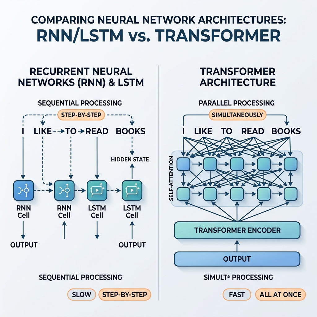
The Parallelization Problem
Because $h_t$ depends directly on $h_{t-1}$, processing cannot be parallelized. To compute the state of the 100th word in a sentence, the network must sequentially compute the first 99 states.
As GPUs and TPUs evolved to support massive parallel matrix computations, this sequential dependency became a critical bottleneck. Training deep RNN models on large web-scale datasets took weeks, whereas the hardware was capable of running much faster if computations were independent.
2. The Information Bottleneck: Vanishing Gradients
As sequence length $N$ increases, backpropagating gradients through time (BPTT) requires repeated matrix multiplication with the recurrence weight $W_{hh}$. If the largest eigenvalue of $W_{hh}$ is less than 1, the gradients shrink exponentially (vanishing gradients). If it is greater than 1, they grow exponentially (exploding gradients).
$$\frac{\partial E_t}{\partial h_1} = \frac{\partial E_t}{\partial h_t} \prod_{k=2}^{t} \frac{\partial h_k}{\partial h_{k-1}}$$
LSTMs and the Memory Constraint
LSTMs introduced the cell state and gating mechanisms (forget gate, input gate, output gate) to allow gradients to flow linearly, mitigating vanishing gradients. However, even LSTMs struggle with sequences longer than a few hundred tokens. The hidden vectors are forced to compress the history of all previous tokens into a fixed-size representation, leading to a “forgetting” effect.
3. How Transformers Solved the Recurrence Problem
The Transformer discarded recurrence entirely, replacing it with the Self-Attention mechanism. Instead of step-by-step state propagation, Self-Attention allows every token to directly interact with every other token in the sequence simultaneously.
The attention matrix is calculated using:
$$\text{Attention}(Q, K, V) = \text{softmax}\left(\frac{Q K^T}{\sqrt{d_k}}\right) V$$
Here is how the Transformer resolves the RNN bottlenecks:
- Massive Parallelization: Because there are no sequential dependencies between positions, all tokens in the input sequence are processed at the same time. The computational graph is shallow and highly parallelizable, utilizing GPUs to their maximum capacity.
- Constant Path Length: The path length between any two tokens is $\mathcal{O}(1)$. This eliminates the vanishing gradient problem over long sequences, enabling models to easily handle contexts of thousands (or even millions) of tokens.
- Positional Encodings: Since there is no inherent sequence order in self-attention, the Transformer injects Positional Encodings into the input embeddings to preserve word order.
4. PyTorch Sequence Processing Comparison
The code snippet below contrasts the sequential loop design of an RNN cell with the parallel matrix computation of a self-attention layer:
import torch
import torch.nn as nn
import time

batch_size = 32
seq_len = 512
embedding_dim = 128

# Inputs: [batch_size, seq_len, embedding_dim]
x = torch.randn(batch_size, seq_len, embedding_dim)

# 1. Recurrent Processing (RNN Cell)
class CustomRNN(nn.Module):
    def __init__(self, dim):
        super().__init__()
        self.rnn_cell = nn.RNNCell(dim, dim)

    def forward(self, x):
        h = torch.zeros(x.size(0), x.size(2), device=x.device)
        # Sequential loop over time steps (cannot be parallelized)
        for t in range(x.size(1)):
            h = self.rnn_cell(x[:, t, :], h)
        return h

# 2. Parallel Processing (Self-Attention Layer)
class CustomSelfAttention(nn.Module):
    def __init__(self, dim):
        super().__init__()
        self.num_heads = 4
        self.mha = nn.MultiheadAttention(dim, self.num_heads, batch_first=True)

    def forward(self, x):
        # Parallel matrix multiplication across all timesteps
        attn_out, _ = self.mha(x, x, x)
        return attn_out

rnn = CustomRNN(embedding_dim)
attention = CustomSelfAttention(embedding_dim)

# Benchmark RNN Sequential Loop
start = time.time()
rnn_out = rnn(x)
rnn_time = time.time() - start

# Benchmark Self-Attention Parallel Execution
start = time.time()
attn_out = attention(x)
attn_time = time.time() - start

print(f"RNN Time (Sequential loop): {rnn_time * 1000:.2f} ms")
print(f"Attention Time (Parallel matrix): {attn_time * 1000:.2f} ms")
5. Architectural Comparison Summary
| Characteristic | RNN / LSTM | Transformer |
|---|---|---|
| Sequential Operations | $\mathcal{O}(N)$ | $\mathcal{O}(1)$ |
| Computational Complexity per Layer | $\mathcal{O}(N \cdot d^2)$ | $\mathcal{O}(N^2 \cdot d)$ |
| Maximum Path Length | $\mathcal{O}(N)$ | $\mathcal{O}(1)$ |
| Parallelization | Limited / Impossible | Highly Parallelizable |
| Long-range Dependencies | Poor (Forgets) | Excellent (Constant path) |
Conclusion
The shift from RNNs to Transformers was driven by computational efficiency and capacity. By replacing sequential recurrence with parallel self-attention, Transformers unlocked the ability to scale model size and dataset size exponentially. This structural breakthrough paved the way for modern Large Language Models (LLMs) like GPT and Claude, which would have been computationally intractable to train using recurrent architectures.