Understanding Transformer Networks and the Self-Attention Mechanism
In 2017, the artificial intelligence landscape changed forever with the publication of the seminal paper “Attention Is All You Need” by Vaswani et al. The paper introduced the Transformer, a revolutionary neural network architecture that discarded recurrence (RNNs, LSTMs) entirely, opting instead to process sequential data in parallel using the Self-Attention Mechanism.
Today, Transformers power almost all state-of-the-art Large Language Models (LLMs), including GPT-4, Gemini, Claude, and Llama. This blog demystifies the Transformer network and explains how the self-attention mechanism is mathematically and practically implemented.
1. The Bottleneck of Sequential Processing (RNNs vs. Transformers)
Before Transformers, models like Recurrent Neural Networks (RNNs) and Long Short-Term Memory (LSTM) networks were the standard for sequence modeling. However, RNNs process tokens sequentially—one word at a time. To compute the hidden state for the 10th word, the model must first compute the hidden states for words 1 through 9.
This sequential nature introduces two severe limitations:
- No Parallelization: Modern GPUs cannot be utilized efficiently because computations must wait for the previous step to complete.
- Vanishing/Exploding Gradients: Information from early in a long sequence gets compressed and lost by the time the model reaches the end (the bottleneck problem).
Transformers solve both issues. By replacing recurrence with Self-Attention, a Transformer processes the entire input sequence simultaneously, allowing for massive parallelization and a direct path between any two tokens in a sequence, regardless of distance.
2. What is the Self-Attention Mechanism?
Self-attention allows the model to evaluate the relationship between different words in the same sequence. Instead of processing a word in isolation, the model represents each word by taking context from all other words in the sentence.
For example, in the sentences:
- “The bank of the river was muddy.”
- “The money was deposited in the bank.”
The word “bank” has different meanings depending on context. Self-attention allows the model to look at “river” in the first sentence and “money” in the second to correctly adjust the representation of “bank”.
The Database Analogy: Queries, Keys, and Values
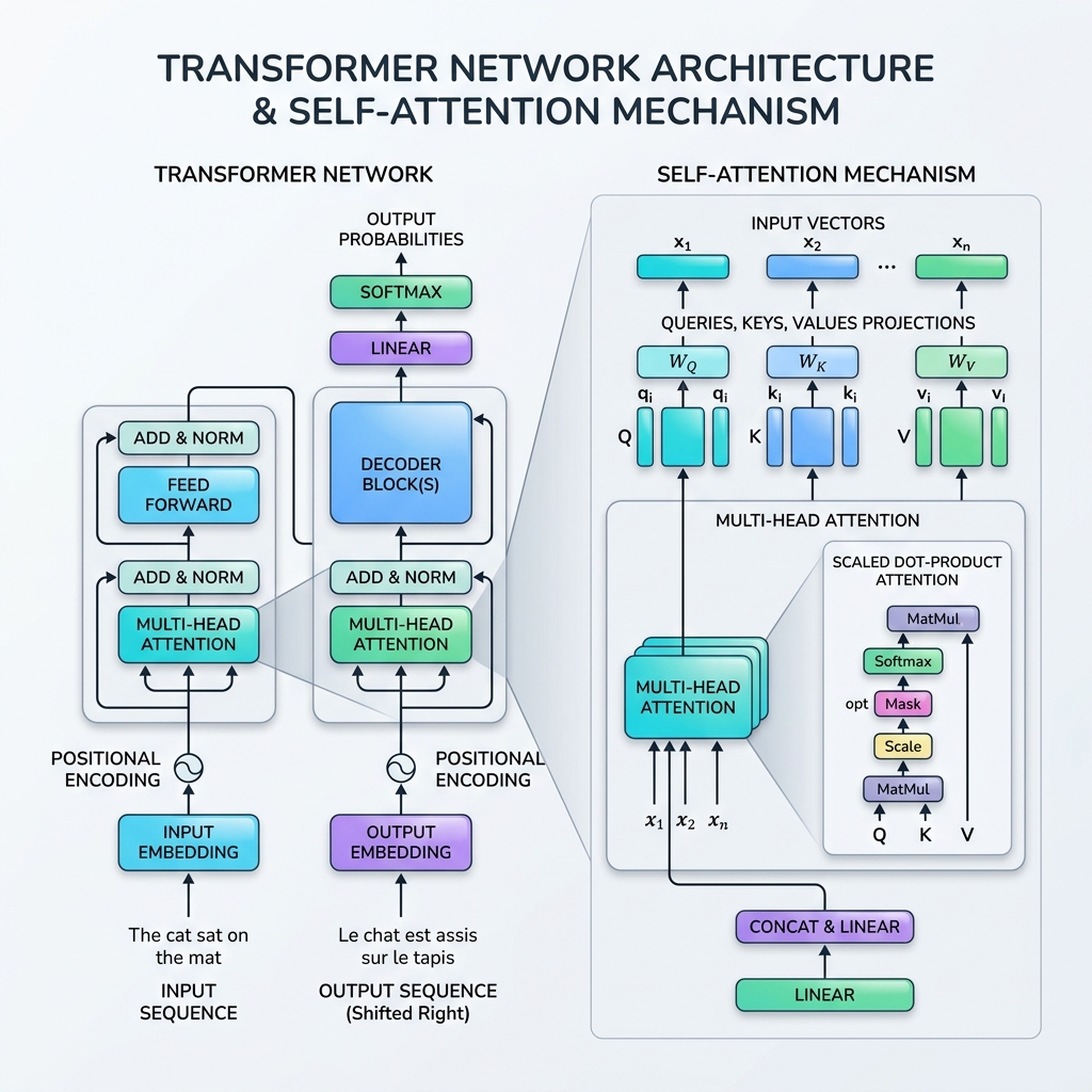
The mathematical formulation of self-attention is modeled after information retrieval (database) lookups. For each input token, we project three vector representations:
- Query ($Q$): What the current token is looking for.
- Key ($K$): The label or profile of the tokens in the sequence.
- Value ($V$): The actual content or information of the tokens.
The attention mechanism computes a similarity score between a Query and all Keys, normalizes these scores into weights, and returns a weighted sum of the Values.
3. Mathematical Walkthrough of Scaled Dot-Product Attention
The standard formula for self-attention is called Scaled Dot-Product Attention:
$$\text{Attention}(Q, K, V) = \text{softmax}\left(\frac{QK^T}{\sqrt{d_k}}\right)V$$
Here is the step-by-step mathematical breakdown of how this formula executes:
Step 1: Compute Projection Matrices
For an input sequence matrix $X \in \mathbb{R}^{T \times d_{\text{model}}}$, we multiply by learnable weight matrices $W_Q, W_K, W_V$ to obtain the Queries ($Q$), Keys ($K$), and Values ($V$): $$Q = X W_Q, \quad K = X W_K, \quad V = X W_V$$
Step 2: Calculate Similarity Scores (Dot Product)
We compute the dot product of the Query matrix $Q$ with the transpose of the Key matrix $K^T$ to measure the raw alignment/relevance between all token pairs: $$\text{Scores} = QK^T$$ The resulting matrix has dimensions $T \times T$, where entry $(i, j)$ represents how much attention token $i$ should pay to token $j$.
Step 3: Scale the Scores
The scores are divided by the square root of the key dimension ($d_k$): $$\text{Scaled Scores} = \frac{QK^T}{\sqrt{d_k}}$$ Why scale? If $d_k$ is large, the dot products grow large in magnitude, pushing the softmax function into regions with extremely small gradients (vanishing gradient problem). Scaling by $\sqrt{d_k}$ stabilizes the training process.
Step 4: Apply Softmax (Attention Weights)
We apply a softmax function along each row to normalize the scores into a probability distribution (values between 0 and 1 that sum to 1): $$\text{Attention Weights} = \text{softmax}\left(\frac{QK^T}{\sqrt{d_k}}\right)$$
Step 5: Weighted Sum of Values
Finally, we multiply the attention weights by the Value matrix $V$: $$\text{Output} = \text{Attention Weights} \times V$$ This step aggregates the information, allowing each token’s output representation to be heavily influenced by the tokens it “attended” to.
4. Multi-Head Attention
Instead of performing self-attention once, the Transformer uses Multi-Head Attention. It splits the Query, Key, and Value vectors into $h$ smaller dimensions (heads), performs attention on each subspace independently in parallel, and then concatenates the results.
This is critical because it allows the model to attend to different types of relationships simultaneously. For instance, one head might focus on subject-verb agreement, while another head focuses on pronoun resolution or temporal references.
5. Python/NumPy Implementation of Attention
To understand the implementation, let’s write a simple, self-contained Python simulation of Scaled Dot-Product Attention and Multi-Head Attention using NumPy:
import numpy as np

def softmax(x):
    # Stabilized softmax to avoid overflow
    exp_x = np.exp(x - np.max(x, axis=-1, keepdims=True))
    return exp_x / np.sum(exp_x, axis=-1, keepdims=True)

def scaled_dot_product_attention(Q, K, V, mask=None):
    """
    Computes Scaled Dot-Product Attention.
    Q: [batch_size, seq_len, d_k]
    K: [batch_size, seq_len, d_k]
    V: [batch_size, seq_len, d_v]
    mask: Optional binary mask [batch_size, seq_len, seq_len]
    """
    d_k = Q.shape[-1]

    # Step 2 & 3: Compute dot-product and scale
    scores = np.matmul(Q, K.swapaxes(-2, -1)) / np.sqrt(d_k)

    # Optional Masking (e.g. Causal masking in Decoders)
    if mask is not None:
        scores = np.where(mask == 0, -1e9, scores)

    # Step 4: Apply softmax to get attention weights
    attention_weights = softmax(scores)

    # Step 5: Weighted sum of values
    output = np.matmul(attention_weights, V)

    return output, attention_weights

# --- Execution Example ---
if __name__ == "__main__":
    np.random.seed(42)
    batch_size = 1
    seq_len = 4  # e.g. "I love deep learning"
    d_k = 8
    d_v = 8

    # Generate random Query, Key, and Value vectors
    Q = np.random.randn(batch_size, seq_len, d_k)
    K = np.random.randn(batch_size, seq_len, d_k)
    V = np.random.randn(batch_size, seq_len, d_v)

    output, weights = scaled_dot_product_attention(Q, K, V)

    print("Attention Weights Matrix (Sequence Length x Sequence Length):")
    print(np.round(weights[0], 4))
    print("\nAttention Output Shape:", output.shape)
6. Architectural Comparison
| Feature | RNN / LSTM | Transformer |
|---|---|---|
| Sequential Processing | Yes (token-by-token) | No (parallelized sequence) |
| Computational Complexity | $O(T)$ sequential | $O(1)$ sequential, $O(T^2)$ total operations |
| Long-Range Dependencies | Poor (memory vanishes over steps) | Excellent (direct link regardless of distance) |
| Parallelization | Impossible along time axis | Native parallelization |
| Positional Awareness | Implicit (inherent in sequential step) | Explicit (requires Positional Encoding) |
7. Additional Transformer Block Components
To make self-attention work in a full stack, the Transformer architecture includes several crucial layers in each block:
- Positional Encoding: Since Transformers process all tokens at once, they have no inherent sense of order. We inject positional encoding vectors (using sine and cosine waves of different frequencies) directly into the input embeddings to represent token order.
- Residual Connections: Skip-connections around each sub-layer (Attention and Feed-Forward) help gradients propagate through very deep networks without vanishing.
- Layer Normalization: Normalizes the activations of each layer, stabilizing and speeding up training.
- Feed-Forward Networks (FFN): A position-wise MLP applied to each token independently, adding non-linear representation capacity.
Conclusion
The Transformer network’s shift from recurrence to parallelized self-attention unlocked the scaling laws of modern AI. By understanding queries, keys, and values, we see how models can dynamically link concepts and construct meaning in real-time, laying the groundwork for the cognitive capabilities of modern LLMs.