Demystifying Sequence-to-Sequence Architecture and the Attention Mechanism
In the landscape of Natural Language Processing (NLP) and Artificial Intelligence, the ability to translate languages, summarize articles, and generate conversational responses has undergone a revolution. At the heart of this transformation lies the Sequence-to-Sequence (Seq2Seq) architecture and the pioneering Attention Mechanism.
Before the advent of modern Transformers, these two innovations solved one of deep learning’s greatest challenges: mapping input sequences to output sequences when their lengths differ.
1. The Foundation: What is Sequence-to-Sequence (Seq2Seq)?
Introduced in 2014 by researchers at Google and others, the Sequence-to-Sequence (Seq2Seq) model is an encoder-decoder framework designed to process sequential data. It is widely used in tasks where the input sequence length does not match the output sequence length, such as:
- Machine Translation: Translating “How are you?” (3 words) to French “Comment allez-vous?” (3 words) or Spanish “¿Cómo estás?” (2 words).
- Text Summarization: Compressing a 500-word article into a 50-word summary.
- Question Answering: Mapping a question sequence to a response sequence.
The Encoder-Decoder Mechanism
The standard Seq2Seq model consists of two recurrent neural networks (RNNs), typically LSTMs (Long Short-Term Memory) or GRUs (Gated Recurrent Units):
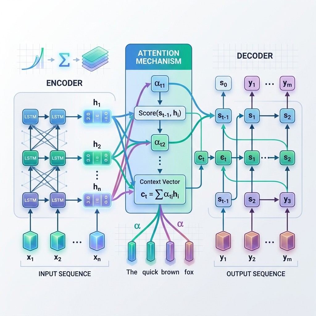
- The Encoder: Processes the input sequence token by token. At each step, it updates its hidden state based on the current input token and the previous hidden state. Once the entire input is processed, the final hidden state of the Encoder is captured. This final state is called the Context Vector (or bottleneck vector).
- The Decoder: Takes the Context Vector as its initial hidden state and generates the output sequence token by token autoregressively. At each step, it predicts the next word based on its current hidden state and the previously generated word.
2. The Bottleneck Problem
While the classic Encoder-Decoder model was a massive breakthrough, it suffered from a fundamental limitation known as the information bottleneck.
In a standard Seq2Seq model, the Encoder is forced to compress the entire meaning of an input sentence—regardless of whether it is 5 words or 100 words—into a single, fixed-size Context Vector.
As a result:
- Long-Term Memory Loss: For longer sentences, the early parts of the sequence are forgotten by the time the Encoder reaches the end.
- Performance Degradation: The quality of translation or summarization drops significantly as the length of the input sentence increases.
Compressing a complex paragraph into a single vector is equivalent to trying to summarize a full chapter of a book in a single sentence before translating it. Information is inevitably lost.
3. The Attention Mechanism: A Paradigm Shift
To solve the information bottleneck, Dzmitry Bahdanau and colleagues introduced the Attention Mechanism in 2015.
Instead of relying solely on a single, static Context Vector from the final step of the Encoder, Attention allows the Decoder to “look back” at all the Encoder’s intermediate hidden states at each step of the decoding process. This means the model dynamically focuses (attends) on different parts of the input sequence depending on the word it is currently generating.
How Attention Works: Step-by-Step
At each decoding step $t$:
- Calculate Alignment Scores ($e_{t, j}$): The model compares the current decoder hidden state $s_{t-1}$ with each encoder hidden state $h_j$ to measure how relevant encoder state $j$ is to the current decoder step. $$e_{t, j} = \text{score}(s_{t-1}, h_j)$$
- Compute Attention Weights ($\alpha_{t, j}$): The alignment scores are normalized using a softmax function to turn them into probabilities (weights) that sum to 1. $$\alpha_{t, j} = \frac{\exp(e_{t, j})}{\sum_k \exp(e_{t, k})}$$
- Generate the Dynamic Context Vector ($c_t$): The context vector is computed as the weighted sum of all encoder hidden states. $$c_t = \sum_j \alpha_{t, j} h_j$$
- Predict the Token: The decoder combines the dynamic context vector $c_t$ with its current state $s_t$ to predict the next output token.
4. Detailed Walkthrough of Seq2Seq and Attention Mechanisms
To truly appreciate the engineering behind these mechanisms, let’s trace the mathematical and operational steps of the classic Sequence-to-Sequence architecture, followed by both Bahdanau (Additive) and Luong (Multiplicative) attention approaches.
Baseline: Classic Sequence-to-Sequence Walkthrough (Without Attention)
Before exploring attention, let’s trace how the standard Sequence-to-Sequence (Encoder-Decoder) architecture processes information sequentially:
- Encoding Phase:
For an input sequence $x_1, x_2, \dots, x_T$:
- At each timestep $t$, the Encoder recurrent cell (LSTM/GRU) updates its hidden state $h_t$ based on the current input token $x_t$ and the previous hidden state $h_{t-1}$: $$h_t = \text{RNN}{\text{enc}}(x_t, h{t-1})$$
- Context Vector Generation:
- The final encoder hidden state $h_T$ acts as the context vector $c$ (the static bottleneck representation): $$c = h_T$$
- Decoding Phase Initialization:
- The Decoder recurrent cell’s initial hidden state $s_0$ is initialized directly with the context vector $c$: $$s_0 = c$$
- Decoder Autoregressive Step:
- At each decoding timestep $t$, the Decoder updates its hidden state $s_t$ based on the previous predicted token $y_{t-1}$ and the previous hidden state $s_{t-1}$: $$s_t = \text{RNN}{\text{dec}}(y{t-1}, s_{t-1})$$
- Token Prediction:
- The probability distribution for the next token $y_t$ is computed using a linear layer and a softmax activation applied to the decoder state $s_t$: $$p(y_t | y_{<t}) = \text{softmax}(W_y s_t + b_y)$$
Approach 1: Bahdanau (Additive) Attention Walkthrough
Bahdanau attention is also called additive attention because it computes the alignment scores using a feed-forward neural network layer. It operates under a “previous-state” dependency flow:
- Initialization / Dependency: At decoding step $t$, the decoder uses its previous hidden state $s_{t-1}$ and the encoder hidden states $h_j$ (for all input steps $j$) to compute attention.
- Calculate Alignment Scores (Additive): $$e_{t, j} = v_a^T \tanh(W_a s_{t-1} + U_a h_j)$$ Here, $W_a$ and $U_a$ are learnable weight matrices that project the decoder state and encoder states into a shared space. Their sum is passed through a $\tanh$ activation function, and then projected to a scalar using the weight vector $v_a$.
- Compute Attention Weights (Softmax): $$\alpha_{t, j} = \frac{\exp(e_{t, j})}{\sum_k \exp(e_{t, k})}$$ This normalizes the alignment scores into a probability distribution over the input sequence.
- Generate Dynamic Context Vector: $$c_t = \sum_j \alpha_{t, j} h_j$$ This is a weighted sum of the encoder hidden states, representing the parts of the input sequence the model should focus on.
- Update Decoder Hidden State: The context vector $c_t$ is concatenated with the embedding of the previous output token $y_{t-1}$, and passed to the decoder recurrent cell to calculate the current decoder state $s_t$: $$s_t = \text{RNN}(s_{t-1}, [c_t; y_{t-1}])$$
- Predict Token: The current state $s_t$ is used to predict the probability of the next token.
Approach 2: Luong (Multiplicative) Attention Walkthrough
Luong attention, introduced shortly after Bahdanau’s, is referred to as multiplicative attention. It simplifies the computation and relies on a “current-state” dependency flow:
- Update Decoder Hidden State First: At decoding step $t$, the decoder first updates its hidden state to $s_t$ using the normal recurrent transition, using only the previous state $s_{t-1}$ and the previous output token $y_{t-1}$: $$s_t = \text{RNN}(s_{t-1}, y_{t-1})$$
- Calculate Alignment Scores (Multiplicative):
Luong proposed three alternative score functions. The most widely used is the General form, which uses a matrix multiplication (hence, multiplicative):
- General: $e_{t, j} = s_t^T W_a h_j$
- Dot: $e_{t, j} = s_t^T h_j$ (assumes equal dimensionality)
- Concat: $e_{t, j} = v_a^T \tanh(W_a [s_t; h_j])$ Multiplicative attention is computationally faster and more space-efficient than additive attention because it can be computed using highly optimized matrix multiplication operations.
- Compute Attention Weights (Softmax): $$\alpha_{t, j} = \frac{\exp(e_{t, j})}{\sum_k \exp(e_{t, k})}$$
- Generate Dynamic Context Vector: $$c_t = \sum_j \alpha_{t, j} h_j$$
- Calculate Attentional Hidden State: Instead of using the decoder state directly for prediction, the context vector $c_t$ and the current state $s_t$ are combined using a linear layer and a $\tanh$ activation to produce an attentional hidden state $\tilde{s}_t$: $$\tilde{s}_t = \tanh(W_c [c_t; s_t])$$
- Predict Token: The attentional hidden state $\tilde{s}t$ is used to generate the final prediction: $$p(y_t | y{<t}, x) = \text{softmax}(W_s \tilde{s}_t)$$
Architectural Comparison
| Feature | Bahdanau (Additive) Attention | Luong (Multiplicative) Attention |
|---|---|---|
| Mathematical Score | Uses a feed-forward network: $v_a^T \tanh(W_a s_{t-1} + U_a h_j)$ | Uses dot product or matrix multiplication: $s_t^T W_a h_j$ |
| Decoder State Used | Uses the previous decoder state $s_{t-1}$. | Uses the current decoder state $s_t$. |
| Computation | More complex, slower but highly flexible. | Faster, simpler, and highly efficient. |
5. The Legacy: From Attention to Transformers
The Attention Mechanism was initially designed as an add-on to enhance RNNs. However, researchers soon realized that the attention layers were doing all the heavy lifting, while the recurrent structures (RNNs/LSTMs) were acting as a computational bottleneck because they had to process tokens sequentially.
In 2017, researchers published the seminal paper “Attention Is All You Need”, introducing the Transformer architecture. The Transformer discarded RNNs entirely, relying solely on Self-Attention to process entire sequences in parallel.
This breakthrough is the foundation of modern Large Language Models (LLMs) like GPT-4, Gemini, and Claude, proving that attention is indeed the single most powerful concept in modern NLP.