How GPT Transformer Works: Causal Self-Attention Explained
In recent years, Generative Pre-trained Transformers (GPT) have revolutionized artificial intelligence. From coding assistants to conversational agents, GPT-based models power the most advanced generative applications today. But how does this technology actually work?
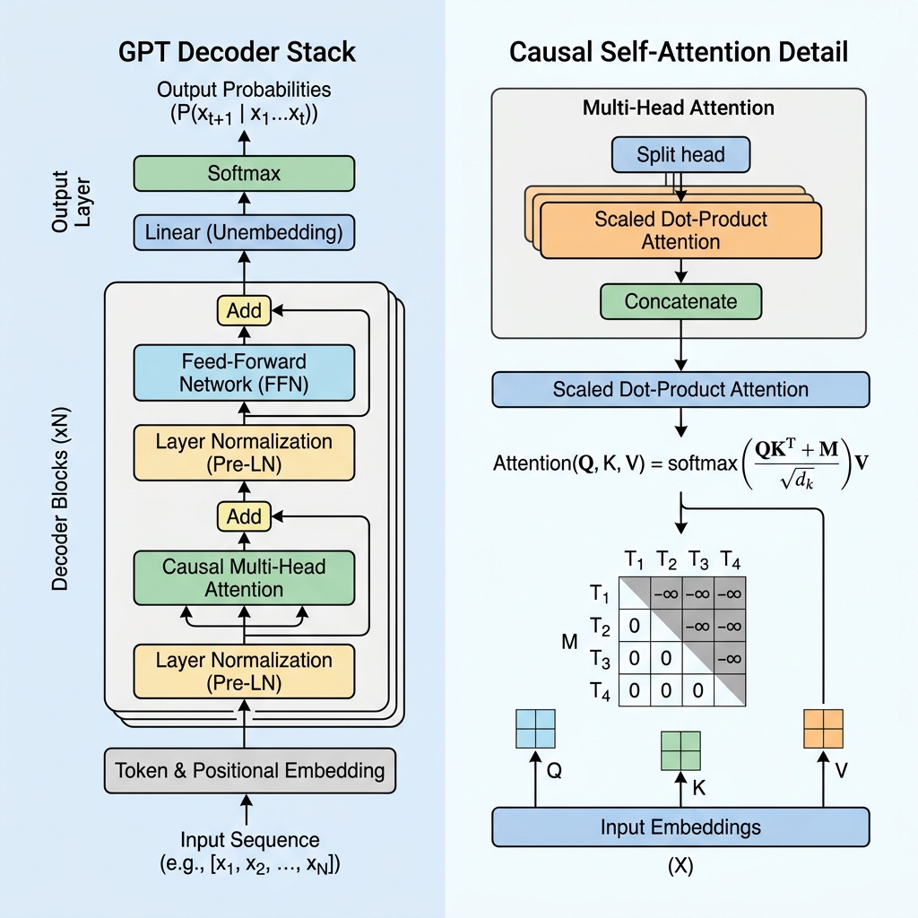
While models like BERT use the Encoder portion of the Transformer to understand text bidirectionally, GPT is a Decoder-only architecture designed for autoregressive, next-token prediction. In this blog, we will demystify how the GPT Transformer works, dive deep into the causal self-attention mechanism, and implement it in code.
1. The Autoregressive Generation Loop
At its core, GPT is an autoregressive model. This means that to generate a sequence of text, it predicts the next token one-by-one, using the tokens it has already generated as context for the next prediction.
The workflow follows these steps:
- Input: The model receives a prompt:
"Deep learning is". - Prediction: The model processes this prompt and outputs a probability distribution over its entire vocabulary. It samples the next token:
"awesome". - Loop: The new token is appended to the input, making it:
"Deep learning is awesome". This sequence becomes the input for the next step. - Termination: The process repeats until the model outputs a special End-of-Sequence (
[EOS]) token or reaches a predefined length limit.
2. Causal Masking: The Heart of the Decoder
In an encoder-only model like BERT, every token can attend to every other token, looking both into the past and the future. However, for a generative model predicting the next token, looking into the future during training would be “cheating”.
To prevent the model from looking at future tokens, GPT uses Causal Self-Attention (or Masked Self-Attention).
The Causal Mask Matrix
During self-attention computation, we calculate similarity scores between tokens by taking the dot product of Queries ($Q$) and Keys ($K$):
$$\text{Scores} = QK^T$$
To enforce causality, we apply a mask matrix $M$ where all values above the diagonal are set to $-\infty$ (negative infinity), and values on and below the diagonal are 0. We add this mask to the scores before applying the softmax function:
$$\text{Masked Scores} = \frac{QK^T}{\sqrt{d_k}} + M$$
$$M = \begin{pmatrix} 0 & -\infty & -\infty & \dots & -\infty \\ 0 & 0 & -\infty & \dots & -\infty \\ 0 & 0 & 0 & \dots & -\infty \\ \vdots & \vdots & \vdots & \ddots & \vdots \\ 0 & 0 & 0 & \dots & 0 \end{pmatrix}$$
When we apply the softmax function, $e^{-\infty}$ becomes $0$. Consequently, the attention weights for any future tokens become exactly 0, rendering future tokens invisible to the current token.
3. Core Architectural Blocks of a GPT Layer
A GPT model consists of stacked Transformer decoder layers. Each layer contains several crucial components:
A. Input Embeddings and Positional Encoding
- Tokenization: Raw text is split into sub-word tokens using Byte-Pair Encoding (BPE).
- Token Embeddings: Each token is mapped to a high-dimensional vector.
- Learned Positional Embeddings: Since self-attention has no inherent sense of order, GPT adds learned positional embedding vectors to the token embeddings, allowing the model to know the position of each token in the sequence.
B. Pre-Layer Normalization (Pre-LN)
Unlike the original Transformer architecture, which applied Layer Normalization after the residual addition (Post-LN), modern GPT architectures apply Layer Normalization before the attention and feed-forward layers:
$$x_{l+1} = x_l + \text{Attention}(\text{LayerNorm}(x_l))$$
Pre-LN stabilizes gradients during training, allowing for the stable training of very deep networks with hundreds of billions of parameters.
C. Feed-Forward Network (FFN)
Following the attention block, the representation of each token goes through a multi-layer perceptron (MLP) consisting of two linear transformations and an activation function (typically GeLU):
$$\text{FFN}(x) = \max(0, x W_1 + b_1) W_2 + b_2$$
4. The Sampling Mechanics (Logits to Tokens)
The final decoder block outputs a vector of raw scores called Logits for each position. We convert these logits into probabilities using the softmax function. To control the randomness of the generated text, we apply parameters during sampling:
- Temperature ($T$): Scales the logits before softmax. A lower temperature (e.g., $T = 0.2$) makes the model deterministic and focused, while a higher temperature (e.g., $T = 0.8$) increases creativity and diversity.
- Top-K: Limits the next token choices to the top $K$ most probable tokens.
- Top-P (Nucleus Sampling): Accumulates the probability distribution and chooses from the smallest set of tokens whose cumulative probability exceeds $P$ (e.g., $P = 0.9$).
5. PyTorch Implementation of Causal Self-Attention
Below is a self-contained PyTorch implementation demonstrating causal self-attention with causal masking:
import torch
import torch.nn as nn
import torch.nn.functional as F

class CausalSelfAttention(nn.Module):
    def __init__(self, d_model, n_heads):
        super().__init__()
        assert d_model % n_heads == 0
        self.d_model = d_model
        self.n_heads = n_heads
        self.d_k = d_model // n_heads

        # Projections for Query, Key, and Value
        self.q_proj = nn.Linear(d_model, d_model)
        self.k_proj = nn.Linear(d_model, d_model)
        self.v_proj = nn.Linear(d_model, d_model)
        self.out_proj = nn.Linear(d_model, d_model)

    def forward(self, x):
        batch_size, seq_len, d_model = x.size()

        # 1. Project inputs to Q, K, V
        Q = self.q_proj(x).view(batch_size, seq_len, self.n_heads, self.d_k).transpose(1, 2)
        K = self.k_proj(x).view(batch_size, seq_len, self.n_heads, self.d_k).transpose(1, 2)
        V = self.v_proj(x).view(batch_size, seq_len, self.n_heads, self.d_k).transpose(1, 2)

        # 2. Compute raw attention scores
        scores = torch.matmul(Q, K.transpose(-2, -1)) / (self.d_k ** 0.5)

        # 3. Create and apply causal mask
        # Upper triangular mask filled with negative infinity
        mask = torch.triu(torch.ones(seq_len, seq_len, device=x.device), diagonal=1).bool()
        scores = scores.masked_fill(mask, float('-inf'))

        # 4. Softmax turns -inf into 0 probability
        attn_weights = F.softmax(scores, dim=-1)

        # 5. Compute weighted sum of values and output
        context = torch.matmul(attn_weights, V)
        context = context.transpose(1, 2).contiguous().view(batch_size, seq_len, d_model)

        return self.out_proj(context)

# Quick verification run
if __name__ == "__main__":
    # Batch size = 1, Sequence length = 4, Model dimension = 8, 2 heads
    x = torch.randn(1, 4, 8)
    attention_layer = CausalSelfAttention(d_model=8, n_heads=2)
    output = attention_layer(x)
    print("Input Shape:", x.shape)
    print("Output Shape:", output.shape)
6. Architectural Comparison
| Feature | BERT (Encoder-only) | GPT (Decoder-only) | Original Transformer |
|---|---|---|---|
| Primary Task | Understanding / Extraction | Generation / Synthesis | Translation / Sequence-to-Sequence |
| Attention Type | Bidirectional Self-Attention | Causal Masked Self-Attention | Bidirectional & Causal Cross-Attention |
| Masking | Masked tokens ([MASK]) |
Causal triangular masking | Causal masking in decoder |
| Processing | Processes whole sequence at once | Autoregressive token generation | Encoder processes once, Decoder generates |
Conclusion
By discarding the encoder and focusing entirely on causal masked self-attention, GPT unlocked the path to generative scaling. The simple rule of predicting the next token, combined with massive parallel training, allows GPT models to capture rich representations of logic, coding, and language, forming the foundation of modern cognitive AI.