Understanding BERT: Bidirectional Encoder Representations from Transformers
In 2018, Google researchers published a landmark paper titled “BERT: Pre-training of Deep Bidirectional Transformers for Language Understanding” (Devlin et al.). This research fundamentally shifted the field of Natural Language Processing (NLP). Before BERT, models processed text sequentially from left to right or right to left. BERT introduced a method to train language representations that look at the context from both directions simultaneously.
Today, BERT and its descendants (like RoBERTa, DistilBERT, and ALBERT) remain foundational for search engines, sentiment analysis, question-answering systems, and information extraction. This article demystifies the BERT architecture, how it works, and how it is trained.
1. What is BERT?
BERT stands for Bidirectional Encoder Representations from Transformers. Let’s break down this name:
- Bidirectional: Unlike traditional language models that read text left-to-right (like GPT) or right-to-left, BERT reads the entire sequence of words at once. This allows it to learn the context of a word based on all of its surroundings (both left and right).
- Encoder Representations: BERT uses the Encoder portion of the original Transformer architecture. It takes an input sequence and outputs a dense vector representation (embedding) for each token.
- Transformers: The underlying engine is the Transformer attention network, which enables modeling of long-range dependencies and parallel computation.
The Power of Bidirectionality
In unidirectional models, a token can only attend to previous tokens. For example, in the sentence:
"He decided to deposit his money in the bank."
If a unidirectional model processes "bank", it only looks at the words before it. But to fully understand the context, looking at both left and right context is crucial. While bidirectional LSTMs attempted this by training separate left-to-right and right-to-left models and concatenating the outputs, BERT trains a single, deeply bidirectional model jointly across all layers.
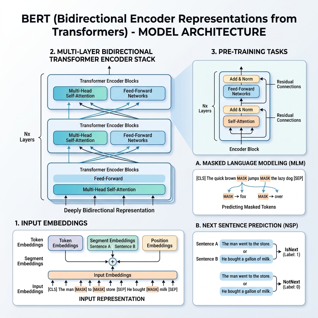
2. BERT’s Input Representation
To enable training on multiple downstream tasks, BERT’s input representation can represent both a single sentence and a pair of sentences (e.g., <Question, Answer>) in a single token sequence.
For any given token, its input representation is constructed by summing three embeddings:
- Token Embeddings: The text is tokenized using the WordPiece vocabulary (about 30,000 tokens). Special tokens are added:
[CLS]: Inserted at the beginning of every sequence. Its final hidden state is used for classification tasks.[SEP]: Used to separate sentences or at the end of a sequence.
- Segment Embeddings: A learned embedding indicating whether a token belongs to Sentence A or Sentence B.
- Position Embeddings: Learned positional vectors added to give the model awareness of the token’s position in the sequence (up to 512 tokens).
$$\text{Input Representation} = \text{Token Embeddings} + \text{Segment Embeddings} + \text{Position Embeddings}$$
3. The Pre-training Process
BERT is pre-trained on a massive corpus (Wikipedia and BooksCorpus) using two unsupervised tasks simultaneously: Masked Language Model (MLM) and Next Sentence Prediction (NSP).
Task 1: Masked Language Model (MLM)
In standard language modeling, predicting the next word restricts models to left-to-right architectures to prevent the target word from “seeing” itself. To train a deep bidirectional representation, BERT randomly masks a percentage of the input tokens and predicts them.
Specifically:
- 15% of the input tokens are chosen at random.
- Of those chosen tokens:
- 80% are replaced with the
[MASK]token. - 10% are replaced with a random word.
- 10% are kept unchanged.
- 80% are replaced with the
This recipe prevents the model from simply focusing only on the [MASK] token during fine-tuning (since [MASK] never appears during fine-tuning) and forces it to build representation vectors for every word in context.
Task 2: Next Sentence Prediction (NSP)
Many downstream tasks (like Question Answering and Natural Language Inference) depend on understanding the relationship between two sentences. To train the model on sentence relationships, BERT is pre-trained on a binary classification task:
When choosing sentences $A$ and $B$ for pre-training:
- 50% of the time, $B$ is the actual next sentence that follows $A$ (labeled as
IsNext). - 50% of the time, $B$ is a random sentence from the corpus (labeled as
NotNext).
The final hidden vector of the [CLS] token is passed to a classification layer to predict the label.
4. Fine-Tuning BERT
One of BERT’s greatest strengths is its flexibility. Pre-training is expensive, but fine-tuning is incredibly cheap and fast. By swapping out the final output layer, BERT can be applied to many different downstream tasks:
- Single Sentence Classification: (e.g., sentiment analysis). Use the
[CLS]token output. - Sentence Pair Classification: (e.g., natural language inference). Use the
[CLS]token output. - Question Answering: (e.g., SQuAD). Predict the start and end span tokens in the document.
- Single Sentence Tagging: (e.g., Named Entity Recognition). Use the output representation of each individual token.
5. Python/Hugging Face Implementation
Below is a simple Python example demonstrating how to load a pre-trained BERT model and extract contextual word embeddings using Hugging Face Transformers and PyTorch:
import torch
from transformers import BertTokenizer, BertModel

# 1. Initialize tokenizer and model
tokenizer = BertTokenizer.from_pretrained('bert-base-uncased')
model = BertModel.from_pretrained('bert-base-uncased')

# 2. Define text containing the word "bank" in two contexts
text_1 = "He deposited money in the bank."
text_2 = "The river bank was muddy."

# 3. Tokenize inputs
inputs_1 = tokenizer(text_1, return_tensors="pt")
inputs_2 = tokenizer(text_2, return_tensors="pt")

# 4. Forward pass through BERT
with torch.no_grad():
    outputs_1 = model(**inputs_1)
    outputs_2 = model(**inputs_2)

# 5. Extract token embeddings
# last_hidden_state shape: [batch_size, sequence_length, hidden_size]
embeddings_1 = outputs_1.last_hidden_state
embeddings_2 = outputs_2.last_hidden_state

# Let's inspect the tokens and their indices
tokens_1 = tokenizer.convert_ids_to_tokens(inputs_1["input_ids"][0])
tokens_2 = tokenizer.convert_ids_to_tokens(inputs_2["input_ids"][0])

# Find the index of the word 'bank'
bank_idx_1 = tokens_1.index("bank")
bank_idx_2 = tokens_2.index("bank")

# Get embedding vectors for the word 'bank'
bank_emb_1 = embeddings_1[0, bank_idx_1]
bank_emb_2 = embeddings_2[0, bank_idx_2]

# Compute cosine similarity
cosine_sim = torch.nn.functional.cosine_similarity(bank_emb_1, bank_emb_2, dim=0)

print("Tokens 1:", tokens_1)
print("Tokens 2:", tokens_2)
print(f"Cosine similarity between both contextual embeddings of 'bank': {cosine_sim.item():.4f}")
6. BERT Model Configurations
Google released two main configurations of BERT:
| Hyperparameter | BERT-Base | BERT-Large |
|---|---|---|
| Number of Layers ($L$) | 12 | 24 |
| Hidden Size ($H$) | 768 | 1024 |
| Attention Heads ($A$) | 12 | 16 |
| Total Parameters | 110 Million | 340 Million |
Conclusion
BERT proved that deep bidirectional representations trained on large unlabeled text can capture complex syntactic and semantic structures. It set a new paradigm for transfer learning in NLP, establishing the pre-train then fine-tune workflow that dominated AI until the rise of autoregressive decoder-only models (like GPT).